Crowded Space, Part 1 of 6
- Almost Orthogonal (this part)
- Superposition
- The Geometry of Superposition
- The Cost of Superposition
- Undoing Superposition
- Open Problems
Almost Orthogonal
How much can a neural network’s space hold?
Table of Contents
- The neural storage problem
- What a space is
- What dimension is
- Vectors and the dot product
- Storing numbers in a space
- Inside a neuron
- Dimension and capacity
- Almost orthogonal
- Ten thousand dimensions
- Try it
- Checking the famous demo
- The threshold at 1/√n
- At the scale of real models
- What I can prove, and what I can't yet
- Predict, then run
- References
The neural storage problem
Here's a strange fact about large language models. A single model knows about millions of things: names, places, languages, programming syntax, old chess openings. But everything it holds at any one point of the text is a single list of a few thousand numbers [1, 15]. Millions of things, a few thousand slots. This series is about how that's even possible, and what it costs.
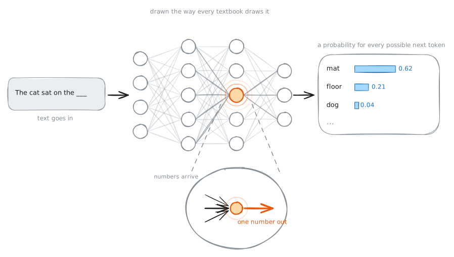
The clearest sign that something odd is happening comes from watching individual neurons. First, two quick definitions, so that nothing here is magic. A language model is a mathematical function: you give it a piece of text, and it gives back a probability for every possible next token, where a token is a word or a piece of a word. Inside, the function has a huge number of adjustable values, and training means tuning those values on enormous amounts of real text until the predictions become good. A neuron is one of the function's smallest parts, and it's a tiny function itself: it takes the numbers flowing through the model and produces a single number of its own. The exact formula is short, and it appears later in this article. For now, the only thing that matters is that watching a neuron means watching one number.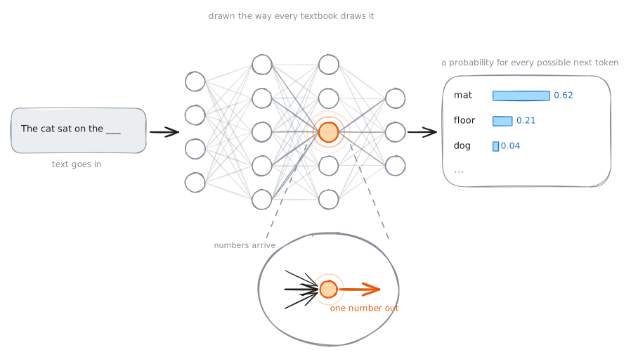
In 2023, researchers at Anthropic trained a small model on purpose: one layer, 512 neurons, small enough to study closely [2]. One neuron's number became large whenever the text was an academic citation. The same number became large on English dialogue. And on HTTP requests. And on Korean text [2]. Four completely unrelated kinds of text, and one number that rises for all of them.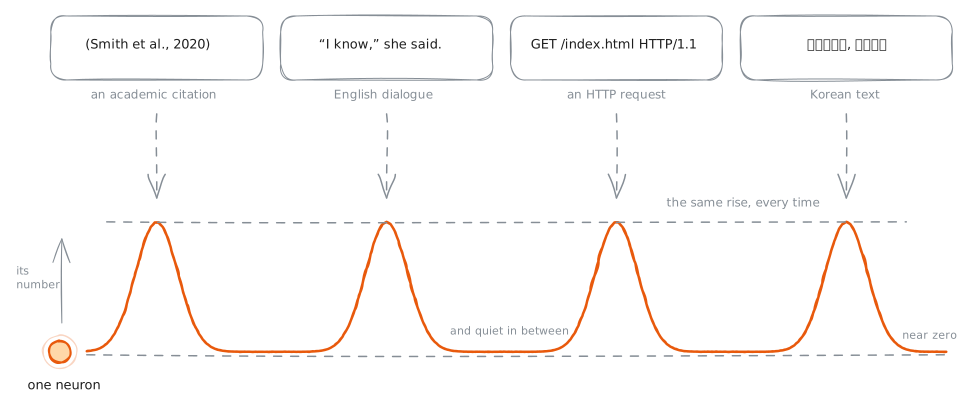
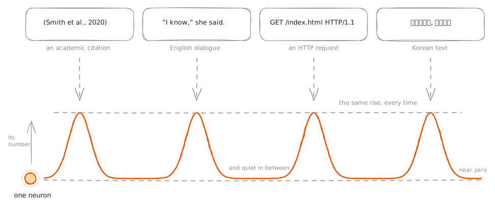
The natural reaction is that the neuron is broken. The model was too small, the training too short.
There's a name for neurons like this, and it comes from Greek: poly, many, sema, meaning. A polysemantic neuron is one unit carrying many meanings at once [2]. And they aren't rare. In large models, polysemantic neurons are the norm, and a neuron with one clean meaning is the exception [2, 3].
Which is why one odd neuron deserves six articles. A model that predicts text well has to track far more things than it has neurons, so sharing isn't optional [1]. And linear algebra, at least the way most of us remember it, says sharing shouldn't work: a space holds only as many independent quantities as it has dimensions. The models clearly didn't read that theorem. Something in the usual understanding of dimension is incomplete.
That gap is what this article is about. Closing it takes four ideas, each rebuilt from the ground: space, dimension, the dot product, and orthogonality. You probably use all four every week. You've probably never had to examine any of them closely. I hadn't either.
One promise before we start. By the end of these six parts, you'll read the research papers this series is built on, Anthropic's superposition papers above all, the way you'd read a colleague's notes. Each part ends by naming exactly which sections of those papers just became readable, so you can check.
What a space is
"Space" might be the most casually used word in mathematics, and it doesn't mean the room around you. A space is a collection of things that we agree to treat as locations. The points of a line are a space. So are the points of a plane, and so is the set of all lists of three numbers. In a few pages, a set of functions will be one too.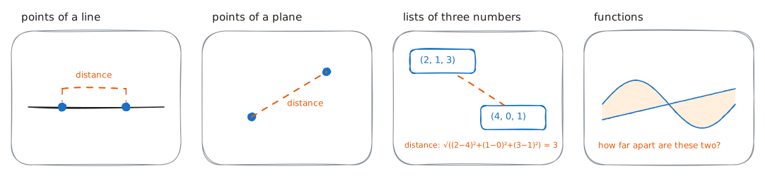
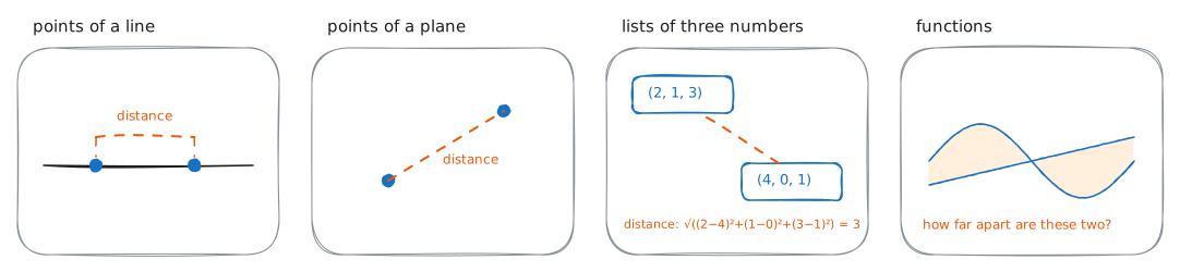
The word is this broad on purpose. Whenever you can point at the members of a collection and say here's one, here's another, you can treat the collection as a space, and once you add a rule for measuring distance, you can do geometry with it. That pattern never changes. Euclidean spaces, metric spaces, every exotic space you'll ever meet: some collection of locations, plus some chosen structure on it.
One distinction is worth fixing early, because it prevents half the confusion people have about dimension. An object is not the space that holds it. A cube gets called "the third dimension" all the time, and it's neither a dimension nor a space. It's a three-dimensional object, one shape out of the infinitely many that three-dimensional space can hold [4]. Objects sit in spaces. The space is everywhere they could be.
What dimension is
The cleanest way I know to build dimension is with motion.
Take a point. It has no length, no width, no depth, just a location. Zero dimensions.
Drag it in one direction, and its path is a line segment, which has length and nothing else. That's one dimension. Drag the segment perpendicular to itself, and it traces a square: length and width, two dimensions. Drag the square perpendicular to its own plane, and you get a cube. Three.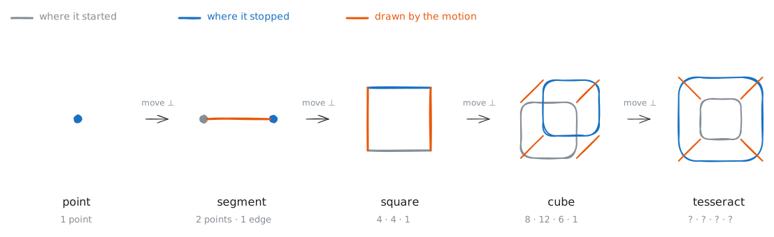
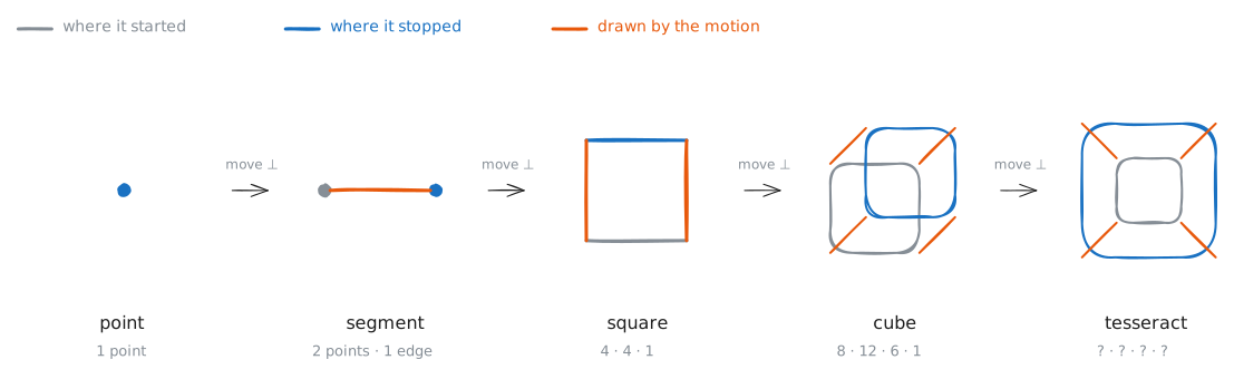
Notice that every step is the same step: move the object perpendicular to every direction it already has. And nothing stops the next one. Drag the cube perpendicular to all three of its directions, and it traces a four-dimensional object called the tesseract. Our world has no room for that motion, and nobody has ever seen a tesseract. But you can still count its parts.
| Object | Points | Edges | Squares | Cubes |
|---|---|---|---|---|
| Point | 1 | |||
| Segment | 2 | 1 | ||
| Square | 4 | 4 | 1 | |
| Cube | 8 | 12 | 6 | 1 |
| Tesseract | ? | ? | ? | ? |
Before you try the last row, test the method on a step you can actually see: the square becoming a cube.
Count the cube's edges. The square's 4 edges sit where the motion started. Another 4 sit where it stopped. And each of the 4 corners drew one new edge as it moved. $4 + 4 + 4 = 12$. A cube has exactly 12 edges, so the method works.
Count the square faces the same way. One square at the start. One at the stop. And 4 new ones, drawn by the 4 moving edges. $1 + 1 + 4 = 6$. Correct again.
That's the whole rule. Every count has three pieces: a copy at the start, a copy at the stop, and one new part drawn by each moving part one level below.
Now the tesseract, by the same rule and nothing else:
- Corners: 8 at the start, 8 at the stop. 16.
- Edges: 12 + 12, plus 8 new ones drawn by the moving corners. 32.
- Squares: 6 + 6, plus 12 drawn by the moving edges. 24.
- Cubes: 1 + 1, plus 6 drawn by the moving squares. 8.
You couldn't see the object, and you counted its parts anyway. All four numbers are exact.
Someone always asks at this point whether the fourth direction is time. In physics it can be. Here it never is: the fourth direction is one more direction of the ordinary kind, exactly as spatial as the first three.
Spaces grow by the same motion as objects. A moving line traces the plane, a moving plane traces our familiar space, and moving all of that in a fourth perpendicular direction gives four-dimensional space. A point in $n$-dimensional space is nothing more exotic than a list of $n$ numbers, and the formulas don't care what $n$ is. For distance, this article uses the standard Euclidean rule, the square root of the sum of squared coordinate differences [4]. There are other distance rules, and two sections from now you'll see where this one actually comes from. From here on, $\mathbb{R}^{n}$ is the usual name for $n$-dimensional space with real coordinates.
And notice that nobody had to give us a definition. It emerged from the construction on its own: the dimension of a space is the number of independent directions in it, or equivalently, the smallest number of coordinates it takes to name a location [4]. Objects have a dimension in the same sense. A sheet of paper in a three-dimensional room is a two-dimensional object, because two numbers are enough to name any point on it.
Two warnings before we continue. Dimension counts independent directions, not things; a line holds infinitely many points and still has exactly one direction. And "I can't imagine ten thousand dimensions" is a statement about human vision, not about the space. You just handled a tesseract without seeing it, and $\mathbb{R}^{10000}$ is no different. The real danger runs the other way, and it's the point of this whole article: the pictures we can see mislead us about the spaces we can't.
Vectors and the dot product
So what's a vector? The honest definition is broader than the arrow you learned to draw. A vector is anything you can do two things with: add it to another of its kind, and scale it by a number. Lists of numbers qualify, added entry by entry, and that makes $\mathbb{R}^{n}$ a vector space whose vectors are the lists themselves. Functions qualify too, since you can add two functions and you can scale one. Remember that; it matters in a few pages.
A list in $\mathbb{R}^{n}$ can be read two ways: as a location, or as a movement, where from any starting point you shift by these amounts along each coordinate. The movement reading is why a vector has a direction. A vector of length one is called a unit vector, and it's pure direction with no size.
The central operation on vectors multiplies matching coordinates and adds everything:
$$\operatorname{dot}(u, v) = u_1v_1 + u_2v_2 + \cdots + u_nv_n$$
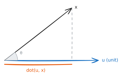
That produces one number, and the number means three things at once, all of them exactly true. Algebraically, it's just the formula: multiply and add. Geometrically, $\operatorname{dot}(u, v) = \operatorname{length}(u) \cdot \operatorname{length}(v) \cdot \cos\theta$, where $\theta$ is the angle between the two vectors [4], so for unit vectors the dot product simply is the cosine of the angle. And there's a third reading, the one this article depends on: when $u$ is a unit vector, $\operatorname{dot}(u, x)$ tells you how much of direction $u$ is present in $x$. You're asking $x$ a question, and the answer is a single number.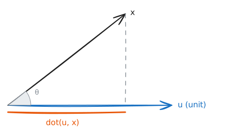
Three terms cause endless confusion around this operation, so let's separate them once and be done. An inner product is any rule $\operatorname{inner}(u, v)$ that turns two vectors into a number while keeping three properties. Order of the inputs doesn't matter. The rule respects addition and scaling in each input. And $\operatorname{inner}(x, x) > 0$ for every nonzero $x$ [5]. The dot product is one member of that family, the most familiar one. And Euclidean space isn't a different set of points at all; it's just $\mathbb{R}^{n}$ once you've chosen the dot product as your rule.
Does the choice matter? The rule $\operatorname{inner}(p, q) = 3p_1q_1 + p_2q_2$ passes all three requirements, so it's a perfectly legal inner product on $\mathbb{R}^{2}$. Under the ordinary dot product, the vector $(1, 1)$ has length $\sqrt{2}$, and the pair $(1, 0), (1, 1)$ sit $45^\circ$ apart. Under the new rule, the same vector has length 2, and the same pair sit $30^\circ$ apart. Same lists, different geometry. Length and angle never belonged to the lists. They come from the rule you choose.
Distance comes from the same choice, since $\operatorname{length}(x)$ is $\sqrt{\operatorname{inner}(x, x)}$ and the distance between two points is the length of their difference. That Euclidean distance rule from the last section? It was the dot product all along.
We'll stay with the plain dot product from here. But the main point stays with us: angle is a chosen measurement, not a given one. And everything ahead is about what happens when angles are allowed to be slightly wrong.
Storing numbers in a space
Orthogonal just means $\operatorname{dot}(u, v) = 0$, which in Euclidean space is the familiar $90^\circ$. Why does anyone care? Because of what it does for storage. Let me show you the whole scheme in two dimensions, with numbers small enough to check by hand. Then we'll give the scheme the opening neuron's job.
Take the plane, and two perpendicular unit directions: $u = (1, 0)$ and $v = (0, 1)$. Say we want one vector to carry two separate quantities, a 3 and a 5. Give each quantity its own direction, scale, and add:
$$x = 3\cdot u + 5\cdot v = (3, 5)$$
One vector now holds both numbers. Reading them back is the question from the last section. Ask $x$ how much of direction $u$ it contains:
$$\operatorname{dot}(u, x) = \operatorname{dot}((1, 0), (3, 5)) = 1\cdot 3 + 0\cdot 5 = 3$$
The reading is 3, exact. Ask with $v$ instead, and the reading is 5, exact. Nothing interfered with anything. The vector is the storage. The dot product is the reading.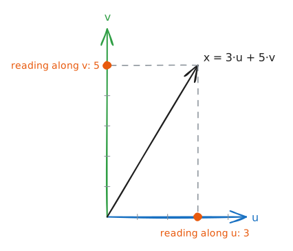
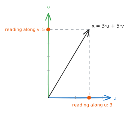
Why did that work so cleanly? Write the reading in general form and watch it, one line at a time. Store an amount $k$ along $u$ and an amount $c$ along $v$, so $x = k \cdot u + c \cdot v$. Then:
$$\begin{aligned} \operatorname{dot}(u, x) &= \operatorname{dot}(u, k\cdot u + c\cdot v) \\ &= k\cdot \operatorname{dot}(u, u) + c\cdot \operatorname{dot}(u, v) \\ &= k + c\cdot \operatorname{dot}(u, v) \end{aligned}$$
The first line is the question applied to what we stored. The second uses the fact that the dot product respects addition and scaling. The third uses $\operatorname{dot}(u, u) = 1$, true for every unit vector. So every reading returns $k$, the number you wanted, plus one extra term: the other amount times the overlap between the two directions. In our example the overlap $\operatorname{dot}(u, v)$ was exactly 0, so the extra term vanished and the reading was perfect.
That extra term has a standard name, interference [1], and it's the cost behind everything in this series.
Now break the scheme, gently. Tilt $v$ toward $u$ until their overlap is $\operatorname{dot}(u, v) = 0.1$. That's a tilt of about $6^\circ$; to the eye, the two directions still look perpendicular. Store the same 3 and 5, and read:
$$\text{reading along } u = k + c\cdot \operatorname{dot}(u, v) = 3 + 5\cdot 0.1 = 3.5$$
You stored 3. You read 3.5. Half a unit of the other quantity leaked into your answer, and nothing in the reading tells you it happened.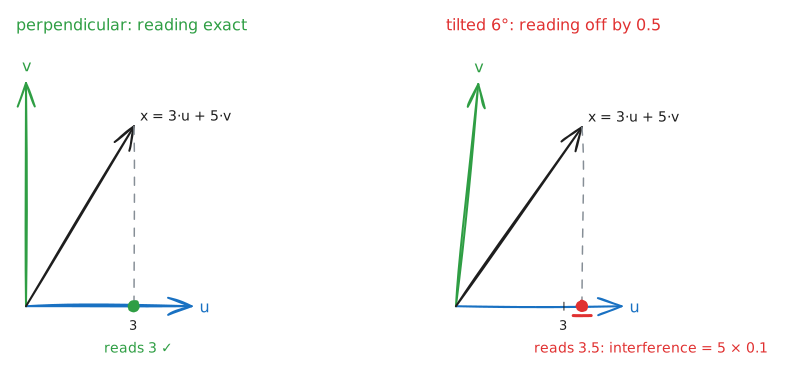
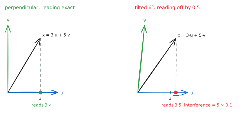
Here's the same leak with meaning attached. Give the two slots the opening neuron's jobs: $k$ is how strongly the current text is Korean, $c$ is how strongly it's an academic citation. Feed the model a pure citation, "(Smith et al., 2020)". The true amounts are $k = 0$ and $c = 5$. With the tilted $v$, the Korean reading is $0 + 5 \cdot 0.1 = 0.5$. The model now holds a signal saying this text is slightly Korean. Nothing Korean exists in the input. The overlap invented it.
The general picture is one step away. In $\mathbb{R}^{n}$ you can pick $n$ directions that are mutually orthogonal, and no more than $n$, because orthogonal nonzero vectors are independent and $\mathbb{R}^{n}$ can hold at most $n$ independent vectors. Store one quantity along each, and every reading is perfect; nothing leaks anywhere. So $n$ dimensions give you $n$ slots of perfect storage, and the supply ends at exactly $n$. That's the sense in which dimension is capacity. Everything ahead either uses that fact or breaks it.
Inside a neuron
Here's the neuron formula I promised.
A neuron holds a vector $w$ (its weights) and a number $b$ (its bias), and training tunes both. Given an incoming vector $x$, it does two things:
$$\begin{aligned} \text{linear step:} \quad & s = \operatorname{dot}(w, x) + b \\ \text{nonlinear step:} \quad & \text{output} = \max(0, s) \end{aligned}$$
The output is called the neuron's activation. With this design it's never negative, and when it's above zero, people say the neuron is active on that input. The cutoff has a name you'll meet everywhere in the literature: ReLU, for rectified linear unit [6]. It isn't the only cutoff in use; many modern models prefer a smoothed relative called GELU [6]. Nothing here depends on which one a model uses, because the pattern is always the same: a linear step, then a simple nonlinear one. A full layer is just many neurons doing this to the same $x$ at once; stack the weight vectors as rows of a matrix, and all the dot products happen in one multiplication.
Now look where $x$ enters: one place, inside $\operatorname{dot}(w, x)$. Everything the neuron will ever learn from $x$ comes through that single dot product, and the cutoff afterward can only reshape what the dot product already measured. So the sentence from the opening, "the neuron's number became large on Korean text," means exactly this and nothing else: on those inputs, $\operatorname{dot}(w, x) + b$ is large.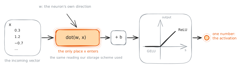
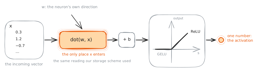
And here's where the two halves of this article meet. Our storage scheme read quantities back with dot products. The network reads its own vectors with dot products, because that's the only reading a neuron performs. Whatever a model stores in $x$, the next layer can use only what a dot product can recover. Storage along directions isn't a modeling convenience somebody chose; the architecture forces it. That's why people study meaning in neural networks as directions [7], and it's why this series does too.
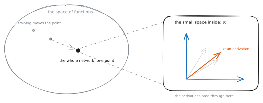
A network is layers of these units, and its overall output is one function built from all of them.
Which means there are two spaces in this story, and they shouldn't be confused. Since functions are vectors, the whole network is a single point in a space of functions, and training moves that point. The storage problem lives in the other space, the small one inside: the $\mathbb{R}^{n}$ that the intermediate vectors, the activations, pass through on their way to the output.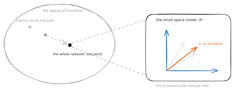
Dimension and capacity
Now I can show you the exact spot where a true theorem turns into a false belief.
The theorem: in $n$ dimensions, at most $n$ nonzero vectors can be mutually orthogonal. Grant Sanderson (3Blue1Brown) gives its status exactly: "to a mathematician, actually, this is the definition of dimension" [6].
The belief: a space holds only as many ideas as it has dimensions. A 300-dimensional word-embedding space (a space where each word is stored as a vector) holds 300 word-features, a 4096-dimensional model space holds 4096 concepts, and that's the end of it.
Here's the strange part: nobody actually states the belief. No textbook prints it, and no theorem proves it. It just forms, quietly, because it feels like a restatement of things that are true. Orthogonal directions stop at $n$. Perfect storage stops at $n$ quantities. So capacity must be $n$. I carried that belief for years without once looking at it directly.
So let's look at it directly. Put the theorem and the belief side by side, word for word: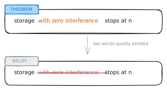
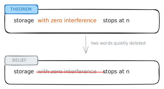
Same sentence. Two words deleted. Nobody performed the deletion on purpose; it happened silently, somewhere between the course and the memory of the course. And the deleted words are not decoration. They are a condition. Our storage scheme told you exactly what stands behind them: every reading returns $k$ plus $c \cdot \operatorname{dot}(u, v)$, and "zero interference" is the demand that the extra term be exactly zero, every time. The belief keeps the conclusion and forgets the condition. It silently assumes that a reading is worthless unless it's exact.
Mathematics offered us exactness. Somewhere we decided meaning requires it. But nobody ever asked the question the deleted words were guarding: how exact does a reading actually need to be?
What if the answer is not "perfectly"?
Almost orthogonal
So allow a small leak. Instead of demanding $\operatorname{dot}(u, v) = 0$ for every stored pair, demand only that it stays small: no bigger in size than some tolerance $\varepsilon$, say 0.05. The reading formula says exactly what this costs. Here it is again:
$$\operatorname{dot}(u, x) = k + c\cdot \operatorname{dot}(u, v)$$
The overlap $\operatorname{dot}(u, v)$ can now be as large as $\varepsilon$, so a reading can be off by at most $c \cdot \varepsilon$: the stored amount times the tolerance. Keep $\varepsilon$ small and every reading stays nearly exact. In angle terms, $\varepsilon = 0.05$ keeps every pair of directions within about $3^\circ$ of perpendicular.
What does the tolerance gain? In the plane, you can check by hand. Two directions at $90^\circ$ satisfy the rule easily; their dot product is exactly zero. Now try a third. It must stay within $3^\circ$ of perpendicular to both. But the first two are perpendicular to each other, so any direction nearly perpendicular to the first is nearly parallel to the second. There's no room at all. Try it below; the third arrow has nowhere legal to point.
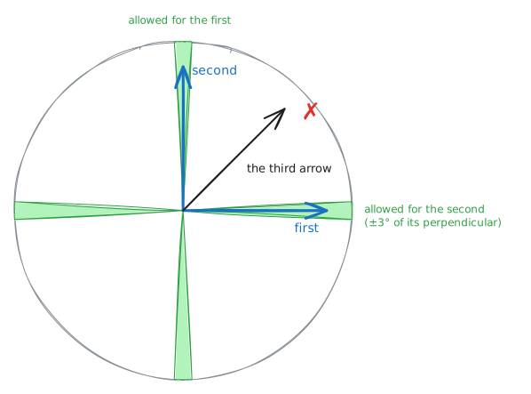
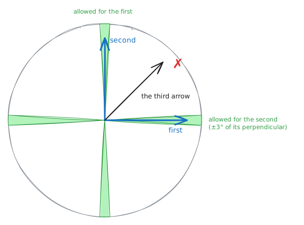
Run the same argument in three dimensions, and you get three directions, exactly what zero tolerance already gave. At this point, the sensible conclusion is that almost-orthogonal is a technicality: it doesn't change how many directions fit. That conclusion is wrong, and it's wrong because two and three dimensions are the wrong place to check it.
Ten thousand dimensions
We can't see $\mathbb{R}^{10000}$. But we can measure it, and the measurement fits in nine lines of code. Here's the plan, before any code.
Pick two directions at random. Record how far from perpendicular they land. Repeat twenty thousand times, so that no single lucky pair can mislead us. Then run the whole experiment in three different dimensions: $n = 3$, a space we can picture; $n = 100$, far beyond anything we can picture; and $n = 10{,}000$, the scale of real models.
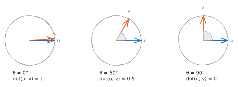
One question first: what number should we record for each pair? The dot product, and here's why it's exactly the right one. Both directions are unit vectors, so $\operatorname{length}(u) = \operatorname{length}(v) = 1$, and the geometric formula from earlier loses both of its lengths:
$$\operatorname{dot}(u, v) = \operatorname{length}(u) \cdot \operatorname{length}(v) \cdot \cos\theta = 1 \cdot 1 \cdot \cos\theta = \cos\theta$$
For unit vectors, the dot product IS the cosine of the angle. No lengths remain in it. So every measurement reads directly as geometry: 0 means exactly perpendicular, $\pm 1$ means parallel, 0.5 means $60^\circ$. One number per pair, and each number is an angle, written as its cosine.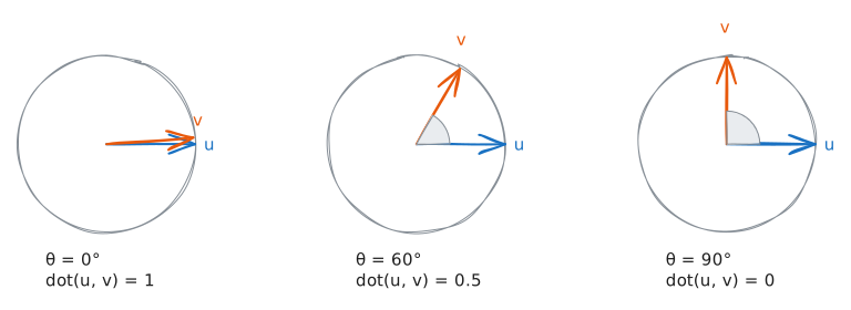
Now the code. Every line states its purpose in its comment.
import numpy as np
rng = np.random.default_rng(seed=1) # fixed seed, so you get my exact numbers
for n in [3, 100, 10_000]: # a space we can see, a middle one, real scale
u = rng.normal(size=(20_000, n)) # 20,000 random vectors...
u /= np.linalg.norm(u, axis=1, keepdims=True) # ...scaled to length 1: directions
v = rng.normal(size=(20_000, n)) # 20,000 more, to form the pairs
v /= np.linalg.norm(v, axis=1, keepdims=True)
dots = np.einsum("ij,ij->i", u, v) # dot(u, v) of each pair, row by row
print(n, round(dots.std(), 4), round(np.percentile(abs(dots), 95), 4))Three details deserve a sentence each. Scaling a random normal vector to length 1 is the standard way to draw a uniformly random direction: the normal distribution has no preferred direction, so after the scaling, every direction is equally likely. And the two printed numbers are two summaries of each batch of 20,000 measurements: the typical size of the dot products (their standard deviation), and the size that 95% of them stay inside. One note on signs: a dot product can be negative, when the two directions lean opposite ways, so the second summary measures size only and ignores the sign.
Here's the output, with the columns labeled, plus one extra column that I'll explain in a moment:
| $n$ | typical size of $\operatorname{dot}(u, v)$ | 95% of pairs stay inside | $1/\sqrt{n}$ |
|---|---|---|---|
| 3 | 0.5799 | $\pm 0.9524$ | 0.5774 |
| 100 | 0.0999 | $\pm 0.1946$ | 0.1000 |
| 10,000 | 0.0100 | $\pm 0.0195$ | 0.0100 |
Now read the table one row at a time. Every dot product here is a cosine, so each one converts to an angle, and I'll do each conversion for you.
Start with $\mathbb{R}^{3}$. The typical dot product is 0.58. Which angle has cosine 0.58? About $55^\circ$. So in three dimensions, that typical size is the cosine of $55^\circ$. Perpendicular would be $90^\circ$. The miss is $35^\circ$, a wide miss. The third column agrees: 95% of pairs stay inside $\pm 0.95$, and since a dot product can never pass $\pm 1$, that's nearly the entire possible range. In plain words: in 3D, a random pair can land almost anywhere, and perpendicular is a special event.
Now $\mathbb{R}^{100}$. The typical dot product is 0.10, and the angle with cosine 0.10 is about $84^\circ$. The typical miss has shrunk from $35^\circ$ to $6^\circ$.
Now $\mathbb{R}^{10000}$. The typical dot product is 0.01, which is the angle $89.4^\circ$. And the third column says 95% of all pairs keep their dot product inside $\pm 0.0195$, which converts to the angle range $88.9^\circ$ to $91.1^\circ$. Within about a degree of perpendicular, for 19 pairs out of every 20.
Say it plainly. Choose two directions at random in ten thousand dimensions, and they're almost certainly almost perpendicular. Nobody arranged that. It's the default state of high-dimensional space.
One column remains: the last one, which the program didn't print. I computed $1/\sqrt{n}$ for each row myself: $1/\sqrt{3} = 0.5774$, $1/\sqrt{100} = 0.1000$, $1/\sqrt{10{,}000} = 0.0100$. Compare it to the second column, row by row. They match to about three decimal places, in every dimension. That's not a coincidence; it's a law. The typical size of $\operatorname{dot}(u, v)$ for random unit vectors is $1/\sqrt{n}$ [11], and your own twenty thousand samples measured it before I ever named it.
Remember that number. It returns twice before the end.
The next page lets you watch all of this happen, live.
Try it
The page asks you for two guesses before it opens, and the guesses are the whole point, so answer honestly. First, as $n$ grows from 2 to 10,000, what happens to the histogram of $\operatorname{dot}(u, v)$ for random pairs? And second, how many directions fit in $\mathbb{R}^{10000}$ if every pair has to keep its dot product inside $\pm 0.05$? Ten thousand? A million? More?
Then drag $n$ and watch. The histogram narrows onto a red curve, which is the exact distribution, with width $1/\sqrt{n}$ at every $n$. The largest dot product in the sample shrinks along with it. And the capacity counter changes its behavior at one sharp threshold. The rest of the article proves what the page shows.
Checking the famous demo
For years I repeated a claim you've probably met too: "the number of almost-orthogonal directions grows exponentially with dimension; this follows from the Johnson–Lindenstrauss lemma." Versions of that sentence appear in the 3Blue1Brown video [6] and in Anthropic's Toy Models paper [1], and I absorbed it from them like everyone else. While preparing this series, I finally checked. Two problems appeared, one small and one large.
The small one is a naming error. The Johnson–Lindenstrauss lemma is about preserving distances: a fixed set of points can be projected into surprisingly few dimensions while approximately keeping every pairwise distance [12]. It's a beautiful fact, but it answers a different question. It never counts how many directions fit, and counting is exactly what we need. The counting question belongs to a different field, the study of sphere packings and spherical codes [13]. Mostly the mislabeling is harmless.
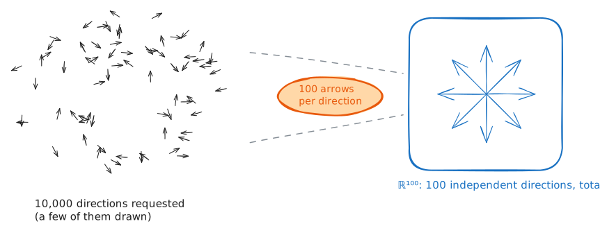
The large problem is the numbers. The video demonstrates the exponential claim with an experiment: 10,000 vectors in $\mathbb{R}^{100}$, adjusted step by step until, as the narration puts it, all pairwise angles sit between 89 and 91 degrees [6].
Before any theorem, hold those two numbers apart and look at them. The space has exactly 100 independent directions; that is what dimension means. The demo asks it to hold 10,000 directions, every pair nearly perpendicular. That's one hundred arrows for every direction the space actually has.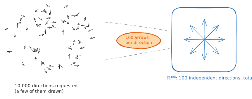
I wanted to reproduce it, and a theorem from 1974 stopped me. The theorem is called the Welch bound [14], and it's about exactly the kind of attempt the video made. Here is that attempt, described slowly.
You have a space with $n$ dimensions. You place $m$ unit vectors in it, in any arrangement you want: random, careful, computed by a machine. Your aim is that every pair be as close to perpendicular as possible.
Whatever your arrangement, examine all its pairs and find the two vectors that lean together the most: the pair furthest from perpendicular. Call it the most crowded pair. That one pair is the honest measure of the whole arrangement, because every other pair is at least as good.
One more step before the theorem, so that every word of it can land. Fix the direction of good and bad. What you want, for every pair, is a dot product near 0, because 0 means perpendicular. The bigger a pair's dot product, the more the two vectors lean together, and the worse that pair is for you. So improving an arrangement means exactly one thing: pushing dot products down, toward 0. Keep that direction in mind; the theorem is about how far down the pushing can go.
Welch proved that the pushing has a limit. In every arrangement of $m$ unit vectors in $n$ dimensions, the most crowded pair's dot product is at least
$$\sqrt{\dfrac{m - n}{n\cdot(m - 1)}}$$
where $m$ is how many vectors you placed and $n$ is the dimension.
What does that mean? Something you can picture directly. A space with $n$ dimensions has room for exactly $n$ fully independent directions, and no more. Now place $m$ vectors, with $m$ bigger than $n$. They can't all be independent. Some of them must lean toward others, simply because there aren't enough separate directions for everyone.
Welch measured that forced leaning. His formula takes your two numbers, $m$ and $n$, and produces one number. Suppose, for a moment, that it produces 0.1. What does a dot product of 0.1 look like? These are unit vectors, so every dot product is the cosine of the pair's angle, and $0.1 = \cos 84^\circ$. So the promise, in geometric words: in every arrangement of your $m$ vectors, at least one pair sits at $84^\circ$ or closer.
Watch it across arrangements. A careless one might have its most crowded pair at a dot product of 0.3, which is the angle $73^\circ$: two vectors leaning hard toward each other. A careful one improves that to 0.15, which is $81^\circ$. The best ones approach 0.1, which is $84^\circ$. But no arrangement, ever, pushes its most crowded pair past $84^\circ$, into the last six degrees before perpendicular. That's the theorem. You can move the most crowded pair to a different spot. You can't remove it, and you can't push its angle closer to perpendicular than the formula allows.
The formula itself looks opaque, so check what it says at its edges. Set $m = n$, exactly as many vectors as directions: the numerator $m - n$ is 0, so the promised overlap is 0, and perfect orthogonality is allowed. That's exactly what we proved with the $n$ perfect slots. Now place vectors past $n$: each extra vector makes the numerator grow, so the promised overlap rises. Crowding is not a side effect in this formula; it's the formula's whole content. Finally, push $m$ toward infinity: $(m - n)/(n \cdot (m - 1))$ approaches $1/n$, so the promised overlap climbs toward $1/\sqrt{n}$ and never passes it. Remember that; it returns in the next section. Read this way, the formula says three plain things: perfection is possible up to $n$, every vector beyond $n$ crowds all the rest, and the crowding approaches a fixed level, $1/\sqrt{n}$.
Now, why does any of this matter for the demo? Stay with the supposed number 0.1, which is the angle $84^\circ$, and write the two sides as two plain sentences.
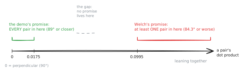
The theorem says: in any arrangement whatsoever, some two vectors sit at 84° or less.
The demo says: in my arrangement, every two vectors sit at 89° or more.
Hold both sentences at once. The same arrangement can't satisfy both, because the two vectors the theorem points at would have to be below $84^\circ$ and above $89^\circ$ at the same time. So if the formula really produces about 0.1 for the demo's $m$ and $n$, then the demo describes an arrangement that cannot exist, and we know it without placing a single vector. Everything now depends on one number: what the formula actually produces for $m = 10{,}000$ and $n = 100$. Let's compute it, one step at a time:
$$\begin{aligned} m - n &= 10{,}000 - 100 = 9{,}900 \\ n\cdot(m - 1) &= 100 \cdot 9{,}999 = 999{,}900 \\ \text{promised overlap} &= \sqrt{9{,}900 / 999{,}900} = \sqrt{0.0099} = 0.0995 \end{aligned}$$
The real number is 0.0995, almost exactly the 0.1 we rehearsed with. So the collision is real. The theorem's sentence: some two vectors sit at $84.3^\circ$ or less. The demo's sentence: every two vectors sit at $89^\circ$ or more. One of these sentences is a theorem, so the other one is false. In every possible placement of ten thousand vectors in $\mathbb{R}^{100}$, some pair stays at least $5.7^\circ$ away from perpendicular. No amount of adjustment can change that.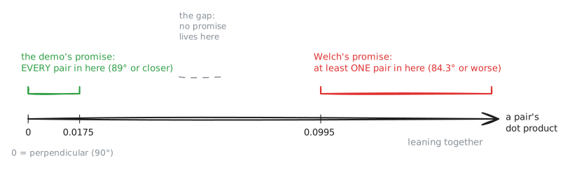
A short argument turns "can't be perfect" into "almost nothing fits." It uses three pieces of linear algebra, and each one can be seen, not just written: a table, its rank, and its trace.
The table first. Take any $N$ almost-orthogonal unit vectors and write the $N$-by-$N$ table of all their dot products: the Gram matrix, whose entry in row $i$, column $j$ is $\operatorname{dot}(u_i, u_j)$ [4]. The diagonal is all 1s, since $\operatorname{dot}(u, u) = 1$. Every other entry is at most $\varepsilon$ in size, tiny. Now set that table next to the $N$-by-$N$ identity matrix, the table with 1s on the diagonal and exact 0s everywhere else. The two are nearly the same picture.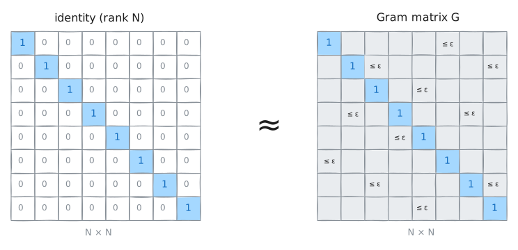
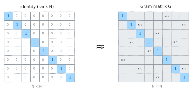
Rank next. The rank of a table is how many of its rows carry genuinely new information. A tiny example: in the table with rows (1, 0, 1), (0, 1, 1), (1, 1, 2), the third row is the first plus the second. It brings nothing new, so the rank is 2, not 3. The identity is the opposite extreme: every row is entirely its own, so the $N$-by-$N$ identity has the maximum possible rank, $N$. And a table that is nearly the identity is nearly full rank.
Now the ceiling. Our table wasn't given to us; it was built from the vectors: $G = V^{\mathsf T} V$, where the columns of $V$ are the vectors themselves. And $V$ has only $n = 100$ rows, one per dimension. A product of two tables can't contain more independence than either factor, so $\operatorname{rank}(G) \le 100$.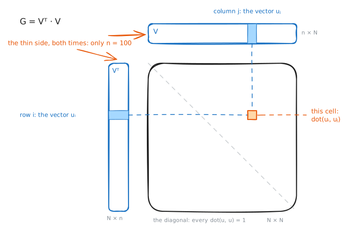
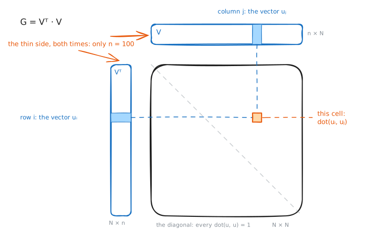
So two facts now stand against each other. The table's shape says: nearly the identity, so rank near $N = 10{,}000$. The table's origin says: rank at most 100. Both can hold only if $N$ isn't actually large. That's the whole proof. What's left is to measure how large $N$ can be, and the measuring tool is the trace.
The trace of a table means: walk down the diagonal and add the entries. Ours is all 1s, so $\operatorname{trace}(G) = N$. No computation, just counting. One more fact, which you may take on faith today or check at home: for any Gram matrix,
$$\operatorname{rank}(G) \ge \dfrac{\operatorname{trace}(G)^2}{\operatorname{trace}(G\cdot G)}$$
(for readers who know eigenvalues: $G$'s are never negative, and this is Cauchy–Schwarz applied to them), and $\operatorname{trace}(G \cdot G)$ equals the sum of every entry of $G$ squared. Count that by hand too: $N$ ones on the diagonal, and at most $N \cdot (N-1)$ other entries no bigger than $\varepsilon$. So $\operatorname{trace}(G \cdot G) \le N + N \cdot (N-1) \cdot \varepsilon^2$. Chain everything:
$$100 \ge \operatorname{rank}(G) \ge \dfrac{N^2}{N + N\cdot(N-1)\cdot\varepsilon^2}$$
and solve for $N$:
$$N \le \dfrac{n\cdot(1 - \varepsilon^2)}{1 - n\cdot\varepsilon^2}, \quad \text{valid whenever } \varepsilon < 1/\sqrt{n}$$
Use the video's own numbers, $n = 100$ and $\varepsilon = \cos 89^\circ \approx 0.0175$: the bound says $N \le 103$. (The general fact behind it, that a nearly-identity matrix must have high rank, is a theorem of Alon [19].)
A hundred dimensions hold at most 103 directions at $89^\circ$–$91^\circ$ tolerance. The famous demo promised ten thousand. The truth is about a hundred times smaller.
And this story has an ending. About a year after the video, Sanderson posted a correction [17]. The demo's code had an error: not every pair actually reached the $89^\circ$–$91^\circ$ range. Some pairs sat near $0^\circ$ or $180^\circ$, hidden at the far edges of the histogram, and the cost function never punished them. A viewer, Nick Yoder, traced the cause and measured the truth: with a repaired loss, ten thousand vectors in $\mathbb{R}^{100}$ reach about $76.5^\circ$ at best, nowhere near $89^\circ$ [18]. Better still, the failed optimization had a structure. It had built roughly one hundred groups of one hundred nearly identical vectors [18]: about one hundred truly distinct directions, each copied about a hundred times. The optimizer knew no theorems, and it found the same ceiling of about a hundred that the table predicted.
I want to be fair to the video, which I admire, and which is how many readers met this question in the first place. Its point stands, and Sanderson said so himself in the correction: the number of almost-orthogonal directions really does grow exponentially with dimension [17]. The demo just sits on the wrong side of a threshold that nobody names. So let's name it.
The threshold at 1/√n
You've now met $1/\sqrt{n}$ twice. It was the typical dot product of random pairs, measured in your own table three sections ago. And it was the condition on the counting bound, whose formula divides by $1 - n \cdot \varepsilon^2$ and is therefore valid only below $\varepsilon = 1/\sqrt{n}$. Twice is not a coincidence. It's one fact, and it's the central fact of this article: $1/\sqrt{n}$ is a border, with a different law on each side. Here's the whole territory on one map, and then a walk through it.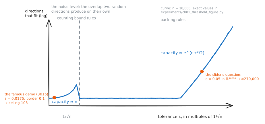
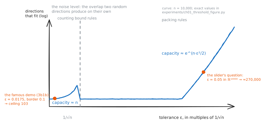
Now the walk, in one concrete space: $n = 10{,}000$, where the border sits at $1/\sqrt{10{,}000} = 0.01$. Keep that number's physical meaning in view. Pick two directions in this space at random, with no design at all, and their dot product is typically about 0.01. The space produces that much overlap on its own. It's the noise level of the space itself.
Start on the map's left side, where the tolerance is below the border. Ask for $\varepsilon = 0.005$, half the noise. Look at what that demand really says: every pair of stored directions must overlap less than two random directions typically do. Randomness itself fails your standard, so no direction comes free, and every new one must be placed against all the previous ones with care. The counting bound measures how far care can go: $N \le 13{,}333$. Exact orthogonality already gave you 10,000 slots. You allowed leaks, and you gained about three thousand more. Barely anything.
Now move to the map's right side. Ask for $\varepsilon = 0.05$, five times the noise. The counting bound can no longer speak here: its formula divides by $1 - n \cdot \varepsilon^2 = 1 - 25$, a negative number, so past the border its derivation fails and it says nothing at all. What replaces it is an argument you can hold in one picture.
Every direction is a point on the sphere: the set of all unit vectors in $\mathbb{R}^{10000}$. When you place a direction, what does it actually forbid? Only the directions too close to it, the ones whose overlap with it would pass $\varepsilon$. On the sphere, those form two small caps: one around the placed direction, and one around its exact opposite, where the overlap is large and negative. And here's the number that decides everything: in high dimensions, the two caps together cover almost nothing, at most $e^{-n\varepsilon^2/2}$ of the surface. (The textbook bound is $e^{-n\varepsilon^2/2}$ for one cap [11]; at our numbers the true cap is more than ten times smaller than that, so the pair fits under the single bound with room to spare.) That smallness is the fact your own table measured: nearly all of the sphere sits almost perpendicular to any one direction. With our numbers that's $e^{-12.5}$, about 3.7 millionths.
So placing directions becomes plain accounting:
$$\begin{aligned} \text{the whole surface:} \quad & 1 \\ \text{forbidden by each placed direction:} \quad & \text{about } 3.7 \text{ millionths} \\ \text{directions placed before the surface is used:} \quad & 1 / (3.7 \text{ millionths}) \approx 270{,}000 \end{aligned}$$
You can keep placing directions until the caps cover the sphere, and that takes about $e^{12.5}$, roughly 270,000 placements. And this is a guarantee, not an estimate of the maximum; the truth is larger still. It's also, at last, the exact answer to the slider's second question.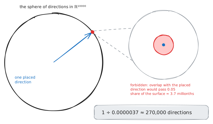
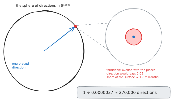
Why is the growth exponential? Because the caps' share, $e^{-n\varepsilon^2/2}$, carries $n \cdot \varepsilon^2$ inside the exponent. Raise the tolerance a little, or the dimension a little, and the share doesn't shrink a little; it shrinks by a factor. Every small increase of the tolerance multiplies the capacity.
One more appearance of the number, and the picture is complete. In the demo section, Welch's promised overlap climbed toward $1/\sqrt{n}$ as $m$ grew, and never passed it. Read that again, now knowing what $1/\sqrt{n}$ is: once there are many vectors, every arrangement, designed by anyone, contains a pair overlapping by about $1/\sqrt{n}$. But a typical random pair already sits at $1/\sqrt{n}$ with no design at all. The cleverest possible placement barely beats random choice.
So one number holds three jobs at once:
- $1/\sqrt{n}$ is the overlap randomness produces on its own.
- $1/\sqrt{n}$ is where the counting bound stops being valid.
- $1/\sqrt{n}$ is the level that the best possible design approaches.
That's the whole section in three lines. And the summary needs no numbers at all. Demand less interference than randomness produces on its own, and you gain nothing. Accept interference at the random level or above, and the space opens exponentially wide.
At the scale of real models
Modern language models are transformers [15]. Each token of the input carries its own vector through the network, and layer after layer, neurons read that vector with dot products and write their results back into it. That carried vector is the residual stream [15], and in a Llama model of the common 7-billion-parameter size, it's a list of 4096 numbers: one vector in $\mathbb{R}^{4096}$. The few thousand numbers from this article's first paragraph are exactly this list.
So the practical question is how many almost-orthogonal directions fit in 4096 dimensions, and the answer depends on the tolerance more than on anything else. At tolerance 0.05, the guaranteed count is about 167, small because 0.05 is only about three times this space's noise level, $1/\sqrt{4096} \approx 0.016$. At 0.10, it's about 800 million. Doubling the tolerance multiplied the guarantee five million times, because the tolerance sits inside an exponent. And randomness alone already delivers: a million random directions fit with every pair between about $83^\circ$ and $97^\circ$, no design needed.
A million meanings in four thousand dimensions. The capacity for the storage problem really exists.
But the geometry can't decide everything by itself, because interference is only paid when it happens. Two overlapping directions collide only when both hold a nonzero quantity at the same moment, and the opening neuron's four meanings almost never share an input; Korean text and HTTP requests rarely arrive together. So the true cost of sharing depends on how often stored things are active at the same time. That property of the world is called sparsity, and it's the whole subject of Part 2.
What I can prove, and what I can't yet
Here's where this leaves us. I can prove that below $1/\sqrt{n}$, interference tolerance gains almost nothing, and capacity stays near $n$. I can prove that above $1/\sqrt{n}$, capacity grows exponentially, that random directions achieve it, and that the Welch bound keeps every arrangement's most crowded pair near $1/\sqrt{n}$. So the capacity for millions of almost-orthogonal directions inside a few thousand dimensions provably exists.
What I can't tell you yet: whether training actually stores meanings along such directions, what geometry it picks if it does, and what the interference costs in practice. Those are Parts 2, 3, and 4.
Predict, then run
Three small predictions before you go. Write each answer down before checking; the prediction is where the learning happens.
The measurement code used $n$ up to 10,000. Using the law you measured, predict the typical size of $\operatorname{dot}(u, v)$ for $n = 1{,}000{,}000$. Then change one line of the code and run it.
In $\mathbb{R}^{4096}$, the guaranteed capacity was about 167 at tolerance 0.05 and about 800 million at 0.10. Before computing: the guarantee is $e^{n\varepsilon^2/2}$, so by what factor does it grow when $\varepsilon$ moves from 0.05 to 0.10? Compute the exponent difference and check your guess.
The counting bound $N \le n \cdot (1 - \varepsilon^2)/(1 - n \cdot \varepsilon^2)$ decided the demo's fate. Use it once yourself: in $\mathbb{R}^{100}$ with $\varepsilon = 0.05$, at most how many directions fit? First predict: closer to 100 or to 1,000? Then compute.
About the sources. The Background & Motivation section of Toy Models of Superposition [1] and the whole of Olah's note on composition and superposition [7] are now fully readable; every idea in them (features as directions, interference, almost-orthogonality) is one you've just used. The 3Blue1Brown chapter [6], together with its correction [17] and the follow-up it inspired [18], will read differently now too. The Demonstrating Superposition section of Toy Models belongs to Part 2, so save it.
If you want more, in rough order of need: Strang's orthogonality chapter or the MIT OCW 18.06 lectures, if $\mathbb{R}^{n}$ feels shaky [4]; Axler's inner-product chapter, for the inner product family done properly [5]; Abbott's Flatland, an 1884 novel about reasoning across dimensions, one evening's read [16]; Cybenko, Hornik, and the Kolmogorov–Arnold paper, if you wonder what stacks of these simple units can represent in principle, a question this article never needed [8, 9, 10]; Vershynin's Chapter 3 and the Dasgupta–Gupta proof of the JL lemma, for the probability machinery [11, 12]; Conway, Hardin and Sloane, for the packing literature itself [13].
The capacity exists. Part 2 asks whether trained networks actually use it.
References
[1] Elhage et al., Toy Models of Superposition, Transformer Circuits Thread, 2022. https://transformer-circuits.pub/2022/toy_model/index.html
[2] Bricken et al., Towards Monosemanticity: Decomposing Language Models With Dictionary Learning, Transformer Circuits Thread, 2023. https://transformer-circuits.pub/2023/monosemantic-features/index.html
[3] Olah et al., Zoom In: An Introduction to Circuits, Distill, 2020. https://distill.pub/2020/circuits/zoom-in/
[4] Strang, Introduction to Linear Algebra, 5th ed., Wellesley-Cambridge Press, 2016. (Orthogonality: Ch. 4.)
[5] Axler, Linear Algebra Done Right, 3rd ed., Springer, 2015. (Inner product spaces: Ch. 6.)
[6] Sanderson (3Blue1Brown), How might LLMs store facts (Deep Learning, Chapter 7), 2024. https://www.youtube.com/watch?v=9-Jl0dxWQs8
[7] Olah, Distributed Representations: Composition & Superposition, Transformer Circuits Thread, 2023. https://transformer-circuits.pub/2023/superposition-composition/index.html
[8] Cybenko, Approximation by superpositions of a sigmoidal function, Mathematics of Control, Signals and Systems, 1989.
[9] Hornik, Stinchcombe & White, Multilayer feedforward networks are universal approximators, Neural Networks, 1989. (For ReLU and every other non-polynomial activation: Leshno, Lin, Pinkus & Schocken, Multilayer feedforward networks with a nonpolynomial activation function can approximate any function, Neural Networks 6(6), 1993.)
[10] Liu et al., KAN: Kolmogorov–Arnold Networks, 2024. https://arxiv.org/abs/2404.19756
[11] Vershynin, High-Dimensional Probability, Cambridge University Press, 2018, Ch. 3.
[12] Dasgupta & Gupta, An elementary proof of a theorem of Johnson and Lindenstrauss, Random Structures & Algorithms, 2003.
[13] Conway, Hardin & Sloane, Packing Lines, Planes, etc.: Packings in Grassmannian Spaces, Experimental Mathematics, 1996.
[14] Welch, Lower bounds on the maximum cross correlation of signals, IEEE Transactions on Information Theory, 1974.
[15] Elhage et al., A Mathematical Framework for Transformer Circuits, Transformer Circuits Thread, 2021. https://transformer-circuits.pub/2021/framework/index.html
[16] Abbott, Flatland: A Romance of Many Dimensions, 1884.
[17] Sanderson (3Blue1Brown), pinned correction comment on [6], 2025. https://www.youtube.com/watch?v=9-Jl0dxWQs8
[18] Yoder, Beyond Orthogonality: How Language Models Pack Billions of Concepts into 12,000 Dimensions, 2025. https://nickyoder.com/johnson-lindenstrauss/
[19] Alon, Perturbed Identity Matrices Have High Rank: Proof and Applications, Combinatorics, Probability and Computing, 2009.